
...
Frequency domain (FD) modelling aims to analyze radio block and circuits response, by assuming an static signal regime (or a particular time period of a dynamic signal) which is integrated infinitely. This simplification allows for simpler & faster mathematical analysis, while still provides an intuitive understanding of the qualitative behavior of the system.
In Radio System Toolbox, FD models of the blocks include the following components:
In the case of passive blocks, noise figure is considered to be inverse to the gain (same magnitude but opposite sign in dB), while OIP3, OIP2 & OP1dB are considered infinite.
Scattering parameters come usually in the form of Touchstone files (*.sNp). These contain the scattering parameters matrix (NxN) of a N-port network as complex values, stored at a number of frequencies. This standard format is the preferred option for most network analyzers, simulation suites & manufacturer data.
You can load Touchstone files to a Radio System Toolbox block, and these will be used to model small-signal FD response of such block.
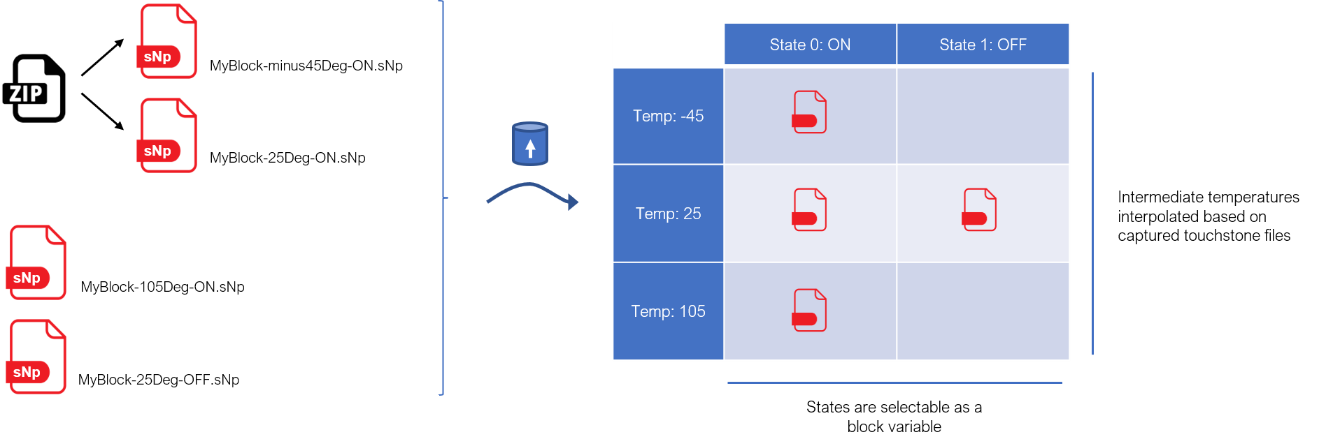
Also, it is usual that models from component manufacturers come as different Touchstone files instead of a single one, for different reasons:
Radio System Toolbox allows for the file upload of multiple S-parameters files in a block, either by multiple selection and/or uploading a zip file. When doing so, an automatic classification of such files will be done based on the names, so that:
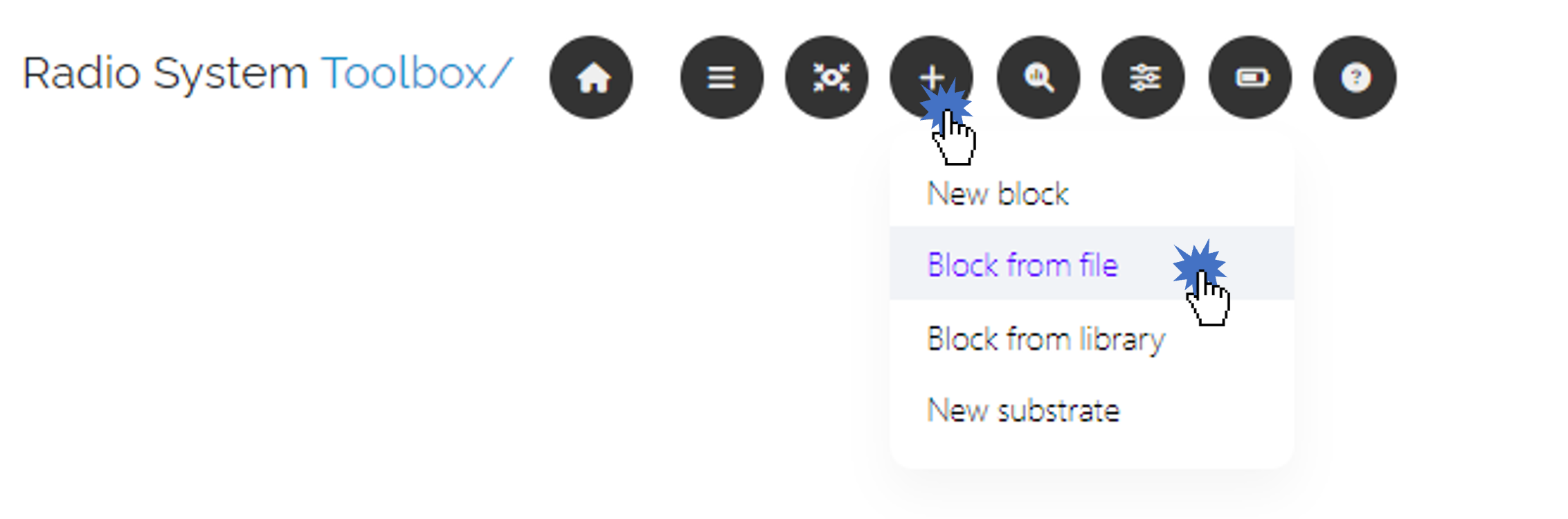
S-Parameter files can be loaded in any of the following ways: * Load files from block dialog
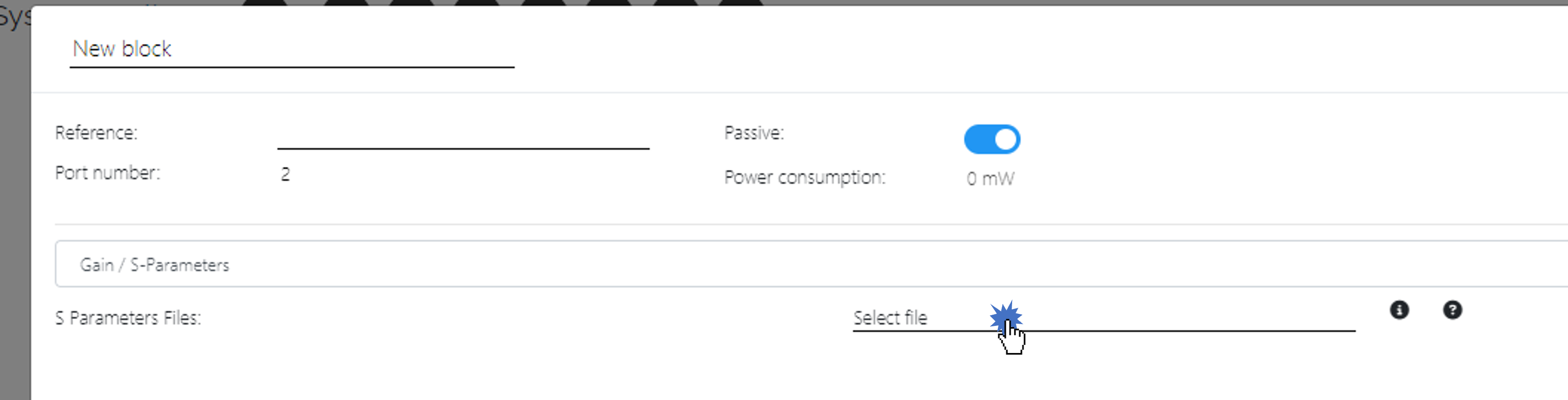
After either of the above actions, a file selector will be opened for you to select the desired files to be uploaded. Once done, they will be classified according to the temperature/state grid, and presented to you.
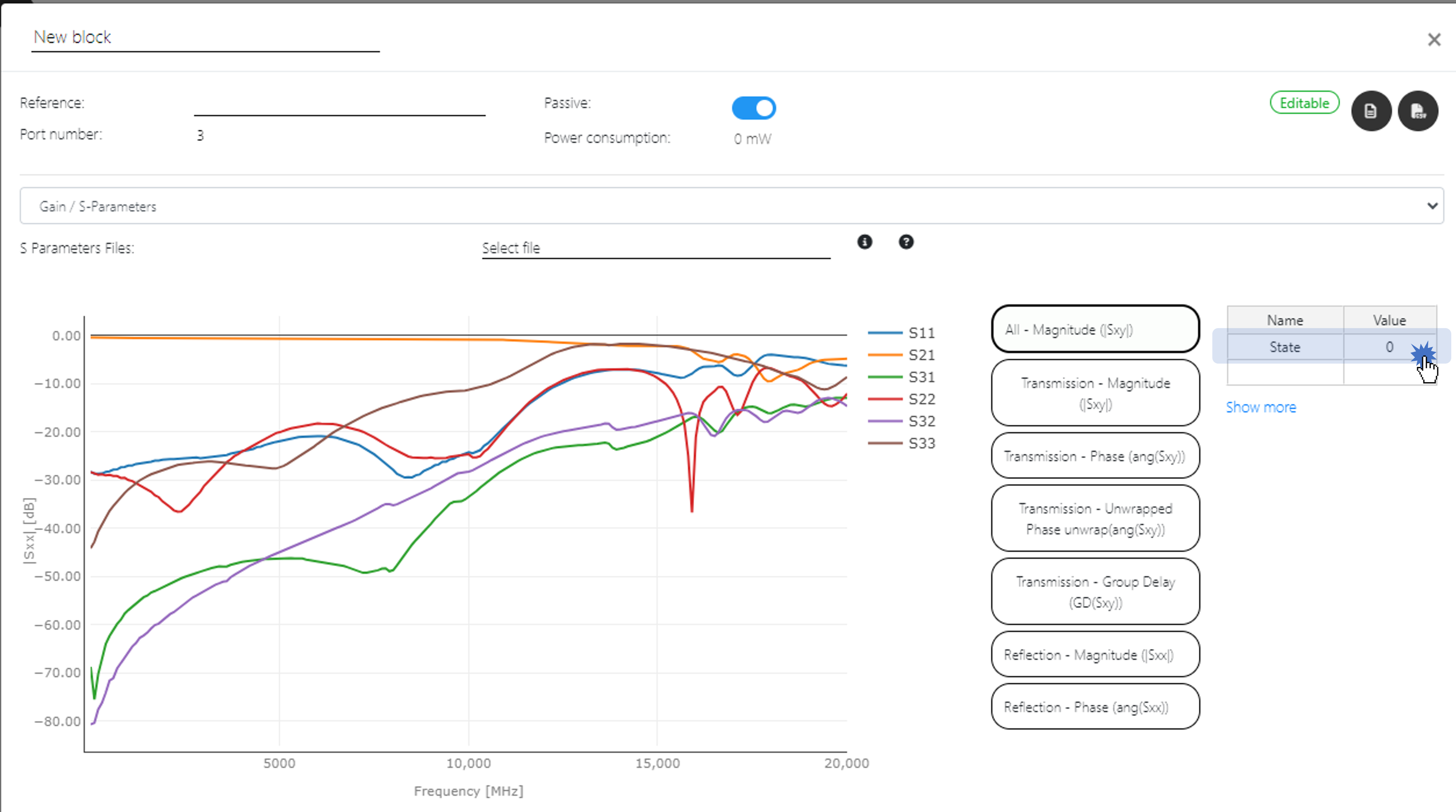
As an example, we uploaded the publicly available model of an SPDT switch (HMC1118 from Analog Devices - S-Parameters File), which comes as a zip file containing S-Parameters for different SPDT switch configurations. They are identified as non-temperature (block states).

After loading, an "State" property is created in the object. By default its value is 0, which corresponds to HMC1118 selection of port RF1 (i.e. common port 0 connected to port 1). S21 is low loss as expected, while S31 shows an isolation of >40 dB,
Changing "State" property to value 2, corresponding to HMC1118 selection of port RF2 inverts the behaviour of S21 and S31 as expected:

Of course, this "State" variable can be swept in a parametric analysis, so that circuit results can be obtained for the different states of each block. For this example, plotting the gain of the circuit path 0 (corresponding to S21) for the different states (0, 1, 2, 3), one can see how this path gain changes as expected.

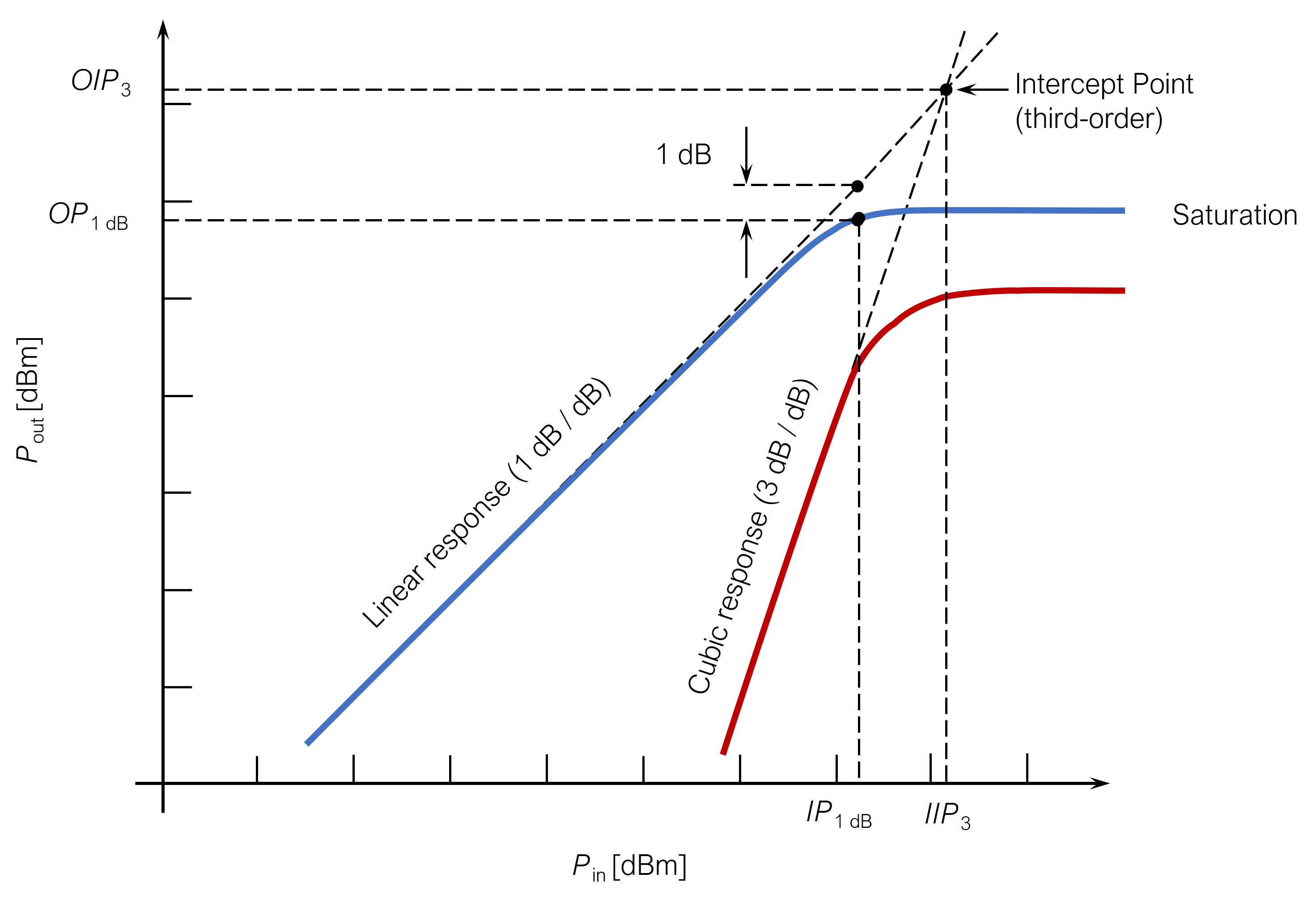
When a block is not defined as passive, the block noise & nonlinearity parameters can be edited in the block dialog. This allows to define Noise Figure, OIP2, OIP3 and OP1dB for different frequencies.
Also, temperature dependency of such parameters can be introduced for each frequency in dB/°C. Once this temperature dependency is defined, the affected noise & performance parameters will be shifted depending on simulation temperature according to this dB/°C slope. The nominal value is considered to be at 25 °C temperature.

Up to the moment, Radio System Toolbox allows for the definition of noise & non-linearity parameters in a single block path (port 1 to port 2). This is fairly enough most active 2-port networks modeling, but of course is limited for some usecases. Further updates might include the capability to define parameters for all block paths.
TO DO: Functionality to derive data from pdf
Radio System Toolbox features several built-in models to be used in simulations. These span from transmission lines to active radio-over-fiber devices, including lumped-element LC filters, attenuators, matching networks, radio propagation models or basic ideal simplified building blocks (like gain blocks, constant losses, etc.)
[7]
...
[8] [9]
...
...
Time Domain (TD) modeling, unlike Frequency Domain (FD), aims to analyze the instantaneous dynamic response of a system for a given excitation (i.e. input signals), without assuming such excitation to be static or periodic.
This approach requires more computing power, and covers usually the characterization of relatively narrowband excitations, yet it can provide some performance metrics which are not achivable by means of FD analysis.
TD block modelling relies first on block FD models data, including S-Parameters and non-linearity figures. Starting from those, incident signals to a block port are processed as follows:
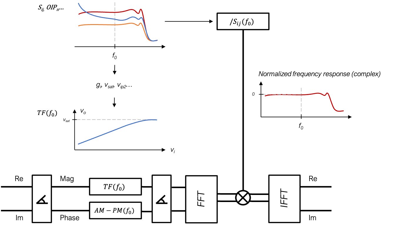
The first processing stage is applied over time-domain complex samples data of the incoming signal, which is changed to polar coordinates (magnitude & phase).
For such processing, the transfer function of the block is calculated based on S-Parameters and non-linearity figures (OP1dB, OIP2, OIP3, OPSat) of the block, for the particular center frequency (f0) of the excitation.
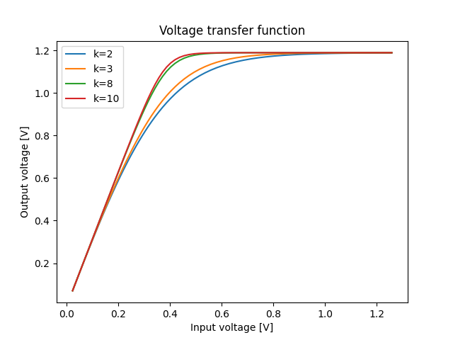
There are different transfer function families that are considered in Radio System Toolbox, although the approach presented by Alfred J. Cann [5], together with a second-order parabolic contribution for modeling OIP2, is used by default.
Following, the calculated transfer function for a block with certain saturation power (OPSat) is depicted following this model [5], for different knee sharpness factors:
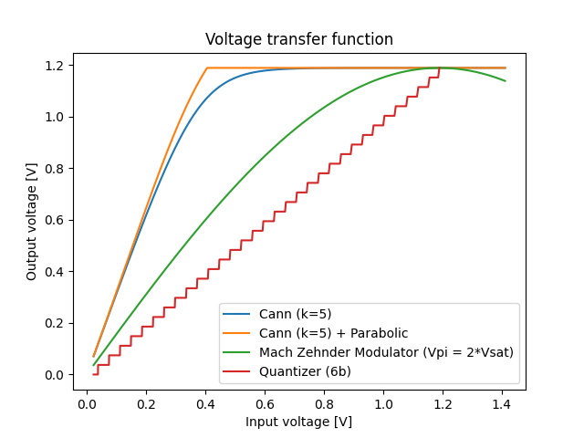
Other transfer function models are used for specific block responses, for example:
As depicted in the above schematic diagram of the TD block model, transfer function is applied over time series such as follows:
After applying the previously explained time-domain sample processing, complex output samples will be already scaled by the block gain and will include non-linearities (such as harmonic distorsion (HD) and intermodulation products (IM)).
Nevertheless, the gain scaling over the samples at this point is referred to the particular center frequency (f0) of the excitation and, given that transfer function is applied at time-domain where no frequency-selectivity exists, it is applied to all frequencies in the signal.
Therefore, there is the need to apply the small-signal frequency response (as defined by complex S-Parameter Sij), after normalizing it respect to Sij(f0). This can be done by a simple frequency-domain multiply, providing FFT and IFFT are applied to the signal before and after.
[1] Times Microwave Systems, "Complete Coaxial Cable Catalog & Handbook, 16th edition". https://timesmicrowave.com/wp-content/uploads/2022/06/tl-16-complete-catalog-r.pdf
[2] Quite Universal Circuit Simulator, Source Code. https://github.com/Qucs/qucsator/blob/develop/src/components/microstrip/msline.cpp
[3] E. Hammerstad and Ø. Jensen, "Accurate Models for Microstrip Computer-Aided Design", Symposium on Microwave Theory and Techniques, pp. 407-409, June 1980.
[4] M. Kirschning and R. H. Jansen, "Accurate Model for Effective Dielectric Constant of Microstrip with Validity up to Millimeter-Wave Frequencies", Electronics Letters, vol. 8, no. 6, pp. 272-273, Mar. 1982.
[5] Alfred J. Cann, Improved Nonlinearity Model With Variable Knee Sharpness, IEEE TRANSACTIONS ON AEROSPACE AND ELECTRONIC SYSTEMS VOL. 48, NO. 4 OCTOBER 2012.
[6] Cox, Charles H., "Analog Optical Links: Theory and Practice". Cambridge University Press 2004.
[7] Pozar, David M. "Microwave Engineering". Wiley; 4th edition (November 22, 2011)
[8] Isao OHTA, Xue-ping LI, Tadashi KAWAI, and Yoshihiro KOKUBO. "A Design of Lumped-Element 3 dB Quadrature Hybrids". 1997 Asia Pacific Microwave Conference
[9] Jian-An Hou and Yeong-Her Wang, "A Compact Quadrature Hybrid Based on High-Pass and Low-Pass Lumped Elements". IEEE MICROWAVE AND WIRELESS COMPONENTS LETTERS, VOL. 17, NO. 8, AUGUST 2007